There is very litte information about Sh2-124 on the Webb. The only information I could find was from the Sharpess Catalogue and Glaxymap.org (here and here). The following is taken from the last of these links.

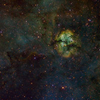
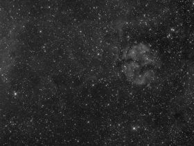
Here's an example. The mysterious HII region Sh 2-124 is located at a distance of about 2600 parsecs towards the north east edge of the Cygnus complex. Almost nothing has been written about this nebula in the scientific literature. In the DSS2 (Digitized Sky Survey) image shown first you can discern a faint amount of nebulosity around the brighter stars. In the far more detailed IPHAS image shown second, however, Sh 2-124 emerges as a spectacular nebula with dividing dust lanes that might be as famous as the Trifid nebula if it were as bright.

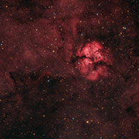
Sh2-124 is fairly bright in Ha and eight hours of exposure picks up a lot of details. The OIII and SII signal is a different matter altogether. On sharplesscatalog Dean Salman writes "I tried the OIII to see if a narrowband was possible, and there just simply is no OIII in this object". However this is not quite true you just need to gather a lot of data. I had to expose for roughly eight hours at 3x3 binning, correspoinding to 72hrs of data at 1x1 binning, in order to get a decent SNR. Even so I had to use a lot of noise reduction to prevent color noise to destroy the image.

Mouseover of the small thumbnails to the left will show the six different combinations of three narrowband images (Ha, OIII and SII).

Hubble Standard: R = SII, G = Ha, B = OIII. The top-left thumbnail is the familiar Hubble composition where the  Ha, OIII and SII images has been adjusted so that they all have similar histograms. In this way the OIII and SII contribution will show up. If this histogram equalization is not done, the image will be dominated by the Ha channel, i.e. it will be green.

Hubble colour shift: The top-middle thumbnail is based on the top-left, to which a colour shift has been applied Photoshop's Selective Color tool (see Bob Frankes tutorial). One has to be very careful when using the Selective Color tool in PS, since it is easy to shift to much resulting in sharp borders between colours.

Hubble modified: The top-right thumbnail is a modification to the Hubble composition (Orange = Ha (hue=35), Red = SII (hue=0), Cyan = OIII (hue=210). Instead of assigning Ha to green I assigned Ha to orange (Hue = 35 in PS notation), SII to red (as in Hubble) and OIII to a slightly more turquoise hue (Hue = 210 in PS notation). This palette has the advantage of separating the different narrowband images (as do the Hubble colour shifting composition), but has the advantage of not being dependent on careful usage of the Selective Color tool.

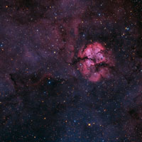
Artificial RGB: The bottom-left thumbnail is an attempt at mapping the narrowband images to colours (R = 80%Ha + 20%SII, G = OIII, B = 85%OIII + 15%Ha) so that the image would mimic the result of a broadband RGB image. It has been constructed by using the fact that H-beta emission (blue) accompanies the H-alpha line (red) with H-beta roughly 15% of the strength of the H-alpha. To the best of my knowledge this was first suggested by Richard Crisp. It also uses the fact that OIII is positioned in-between the blue and green part of the spectra. A litte bit of SII is added to the red channel.

ARGB redder: the bottom-middle thumbnail is based on the Artificial RGB image but the OIII contribution has been dialled down. Sometimes the ARGB blend above gives white areas where OIII is the strongest. In order to get a more "realistic" RGB representation the OIII contribution to both the blue and the green channel can be turned down to your subjective liking.

ARGB bluer: the bottom-right thumbnail is based on the Artificial RGB image but the OIII contribution to the blue channels has been dialled up. One of the ideas behind the Hubble palette representation is that it visualizes the different contributions Ha, OIII, SII. This can also be achieved in a RGB like representation by dialling up the OIII contribution to the blue channel. In this way the OIII areas will be bluish, the Ha areas will be reddish and the SII areas will be deep red.

In order to make most use of the weak OIII and SII data I have also used JP Metsavainio's Tone Mapping technique. A pdf that outlines tone mapping can be found here, and in order to bring out as much details as possible I have followed some of the tutorials on Ken Crawford's site.

Below you see images for each emission line respectively. The images has been stacked and stretched so that the histogram peak is equal for each of them. Note that the binning of the OIII and SII data was  3x3. This mean that each pixel receives 9 times as many photons compared to 1x1 binning. Thus a 8hr exposure would correspond to a 72hr exposure binned 1x1. Binning 3x3 of course looses detail, which in this image has been compensated by constructing a luminance using the H-alpha image with a touch of the OIII and SII data in it (OIII and SII is very weak).

           

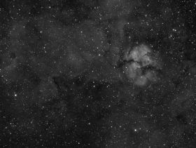
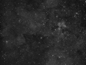
Ha                                                                    OIII                                                                  SII 

The following software has been used. MaximDL (image acquisition and guiding), CCDStack (calibration and RGB scaling, PixInsight (cropping, background correction, colour corrections) and Photoshop CS5 (all the rest, incl Noel Carbonis Astronomy Tools), and finally JP Metsavainio's Tone Mapping technique.

This image was processed in December 2013